Here is the first personal notes from the Reinforcement Learning course that I have decided to take at the MVA Master’s program. The course is quite theoretical and this is challenging for me since I have (almost) zero knowledge on Reinforcement Learning. I have decided to try to explain what I have understood in each lecture in order to assimilate the content of each session.

What is Reinforcement Learning?

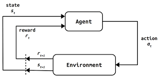
RL is a family of Machine Learning techniques in order to solve a task that is based on the current and previous states of an agent interacting with an environment. In the most practical cases, the agent learns by interacting under uncertainty (i.e. the environment is unknown). In practice, RL can solve several problems related to portfolio management, autonomous driving, game theory and so on.

Probelm statement in RL

In a RL configuration the time needs to be discrete, i.e $t = 1, 2, 3$ thus not continuous. At each time stepm the agent:

• Selects and action based on the current state or on all the states
• Gets a reward
• moves to a new state

Markov Chains and RL

A Markov chain is a dynamic system that satifies the Markov Property:

$$ \begin{equation} \mathbb{P}(s_{t+1} | s_{t}, s_{t-1},…,s_{0}) = \mathbb{P}(s_{t+1} | s_{t}) \end{equation} $$

Also, the transition between each state is determined by a probability called transition probability. In the case of RL, we also consider the space of actions $A$, the transition probability formula becomes:

$$ \begin{equation} p(s'|s, a) = \mathbb{P}(s_{t+1} | s_{t}=s, a_{t} = a) \end{equation} $$

Granularity of the time step

How granular needs to be the time step? The granularity will depend on each problem and needs to be fine-tuned. For e.g., for an Atari game we may need 4 frames between each step in order to notice the direction of the ball to take the optimal decision

Assumptions under a Markov Decision Process

• Each transition needs to be characterized by a reward that can be deterministic or stochastic.
• The dynamics and reward do not change over time

Policies and Decision rules

In order to solve a MDP and find the optimal solution, the final goal for the agents is to learn a Policy that is defined as a set of decision rule. The latest, is a function $d: S \mapsto A$ that takes a state $s \in S$ as an input, and outputs and action $a \in A$. The decision rule can be:

• Deterministic
• Stochastic
• History-dependent
• Markov?

An agent behaving under the policy $\pi$ selects at round $t$ the action: $$a_{t} \backsim d_{t}(s_{t})$$

Optimiality Principles

A metric to ‘evaluate’ a policy is to compute the State Value Function $V^{\pi}$.

If the time horizon is finite

$$V^{\pi}(t, s) = \mathbb{E}[ \sum_{\tau = t}^{T-1} r(s_{\tau}, d_{\tau} (s_{\tau})) + R(s_{T}) | s_{t} = s; \pi = (d_1,…,d_{T})]$$

If the time horizon is infinite

This is used in practice when there is an uncertainty about the deadline.

$$V^{\pi}(s) = \mathbb{E}[ \sum_{t=0}^{\infty} \gamma^t r(s_{t}, d_{t} (s_{t})) | s_{0} = s; \pi = (d_1,…,d_{T})]$$ With $$\gamma \in [0,1)$$

Basically the coefficient $\gamma$ indicates around which time step we should get most of the rewards. If $\gamma$ is small, then the STF will focus on short-term rewards, otherwise the function will flag long-term rewards.

Optimal Value Function

The solution to an MDP is an optimal policy satisfying

$$\pi^{*} \in argmax V^{\pi}_{\pi \in \Pi}$$

It is not an equality since we may have several optimal solutions for the problem. The corresponding value function is the optimal value function $$ V^{*} = V^{\pi^{*}} $$

Q-function

The Q-function is a function that maps from $ S \times A \mapsto \mathbb{R} $

$$ Q^{\pi} (s, a) = \mathbb{E} [ \sum_{t=0}^{\infty} \gamma^t r(s_t, a_t) | s_0 = 0, a_0 = a, a_t = \pi(s_t) ] $$

The Q-function represents the expected reward when we take an action $a$ in the state $s$. It represents the quality of a certain action in a given state.

Bellman operator and Bellman equation

Notations

An example is worth thousands words. In order to define the variables that we are going to use, let’s define a simple MDP which is the one below:

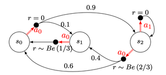
The decision rule $\pi$ is a set of size $N$, with $N$ corresponding to the number of states. Each value of $\pi_i$ corresponds to the action that we take at the state $s_i$. $$\pi = \{\textcolor{#E94D40}{\pi_0},\ …\ ,\ \pi_N \} $$ $$ \textcolor{#E94D40}{\pi_{0\ }}\ \in\ A $$

The transition probabilities matrix can be easily written. Each row $i$ corresponds to the probabilities of moving from a state $i$ to all possible states $j \in {1,..,n}$ given a decision rule $\pi$. Thus here if $\pi$ is stationary and $\pi = \{\textcolor{#E94D40}{a_0},\ \textcolor{#E94D40}{a_0} ,\ \textcolor{#3697DC}{a_1}\}$,

$$ \begin{align} P = \begin{pmatrix} 0 & 0.1 & 0.9 \\\ 1 & 0 & 0 \\\ 0 & 0 & 1 \end{pmatrix} \end{align} $$

The reward vector $r^\pi$ is the vector containing the expected rewards at each state, given a policy $\pi$. In our case, using the same policy, we obtain

$$ \begin{align} r^\pi & = & \begin{pmatrix} 0 \\\ \mathbb{E}(Be(1/3)) \\\ 0 \end{pmatrix} & = & \begin{pmatrix} 0 \\\ 1/3 \\\ 0 \end{pmatrix} \end{align} $$

If $\pi$ was $\{\textcolor{#E94D40}{a_0},\ \textcolor{#E94D40}{a_0} ,\ \textcolor{#E94D40}{a_0}\}$ we would obtain:

$$ \begin{align} r^\pi & = & \begin{pmatrix} 0 \\\ \mathbb{E}(Be(1/3)) \\\ \mathbb{E}(Be(2/3)) \end{pmatrix} & = & \begin{pmatrix} 0 \\\ 1/3 \\\ 2/3 \end{pmatrix} \end{align} $$

Bellman equation

Given a state $s$ and, policy $\pi$ and a set of transition probability, we can analytically compute the value of the Value Function in an exact way using the Bellman Equation.

$$ \begin{equation} V^{\pi}(s)=r(s, \pi(s))+\gamma \sum_{y} p(y \mid s, \pi(s)) V^{\pi}(y) \end{equation} $$

The equation below can be written also in a matrix form:

$$ \begin{align} V^{\pi} &=r^{\pi}+\gamma P^{\pi} V^{\pi} & & \Longrightarrow & V^{\pi} &=\left(I-\gamma P^{\pi}\right)^{-1} r^{\pi} \end{align} $$

which can be easily computed if all the variable were know beforehand, which in practice not really the case since the environment with which the agent interacts is unknown.

Bellman operator

For any $W \in \mathbb{R}^n$, the Bellman operator is a function $\mathcal{T}^{\pi} : \mathbb{R}^n \mapsto \mathbb{R}^n$ such that:

$ \mathcal{T}^{\pi} W(s)=r(s, \pi(s))+\gamma \sum_{s^{\prime}} p\left(s^{\prime} \mid s, \pi(s)\right) W\left(s^{\prime}\right) $

This operator encapsulates the fundamental operation in order to compute a Value Function, given a MDP

When the policy is unknown we use the following formula to compute each component of $W$: $ \mathcal{T} W(s)=\max _{a \in A}\left[r(s, a)+\gamma \sum_{s^{\prime}} p\left(s^{\prime} \mid s, a\right) W(s)\right] $

As you can see, the formula of the Bellman equation isrecursive. In practice, this is computed and solved using dynamic programming.