In the previous section we have seen how to formulate a RL problem using MDPs and provide some tips in order to analytically evaluate a policy (set of actions at each set) if some variables were known beforehand using the Bellman equation and the Bellman operator.

Here in the second lecture we are going to tackle the issue of how to solve an MDP (i.e get the optimal policy $\pi$) given some parameters of the problem. Few techniques exists in order to achieve this, let’s start with the Value Iteration

Value Iteration

Intuition

We have few tools in our toolbox. First of all, how do we evaluate a policy? We can simply compute the Value Function which corresponds to a kind of “summary” of the rewards at each state, given a policy. If we consider again the simple MDP considered last week, if the policy is $\pi = \{\textcolor{#E94D40}{a_0},\ \textcolor{#E94D40}{a_0} ,\ \textcolor{#3697DC}{a_1}\}$

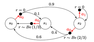
Analytically, The Value Function is equal to $V^\pi = [0.033, 0.363, 0]$. Which means intuitively, that in expectation under the given policy, moving frequently to the state $s_1$ is highly benefic in terms of reward.

What if the policy is unknown? Then the problem would have a different formulation, our goal would be to find the best policy possible among the combination of all possible policies. You can image that this is doable if the problem is simple enough ($|A| < N_A$ and $|S| < N_S$, i.e reasonable number of possible actions and reasonable number of states) but extremely complex if not.

The idea of the Value Iteration algorithm is the following:

• Initialize $V_0$ in $R^N$
• At each iteration $k = 1,2,…,K$:
  • Compute $V_{k+1} = \mathcal{T}V_k$ until $|| V_{k+1} - V_k || \leq \epsilon$
• Get the greedy policy $ \pi_{K}(s) \in \arg \max _{a \in A}\left[r(s, a)+\gamma \sum_{s^{\prime}} p\left(s^{\prime} \mid s, a\right) V_{K}\left(s^{\prime}\right)\right] $

Recall that the greedy policy is $\in$ the set of $argmax$ because we may have several values that reaches the maximum.

Intuitively, the algorithm would work as the followwing

• Initialize with a random Value Function
• Compute the Bellman operator applied to this Value Function for all the possible actions and update $V_k$ at each step by considering the action that maximized the Value Function (i.e. the optimal action)

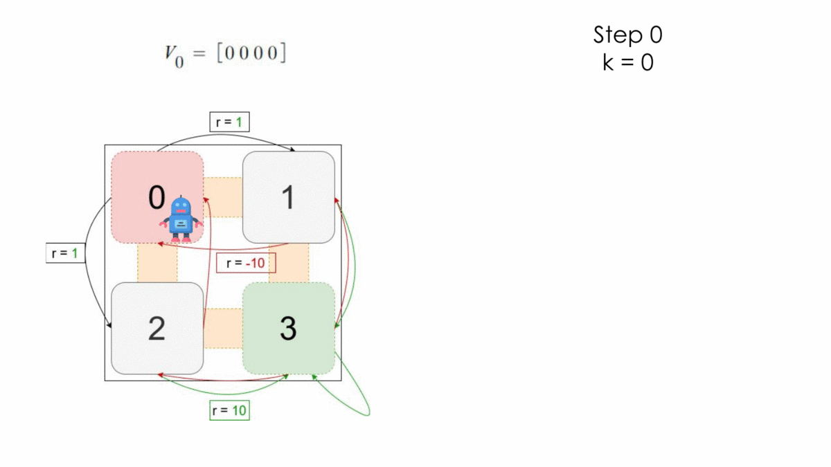
Let’s consider the following problem, where the initial state is $S_0$ and the final state $S_3$. The set of actions here is $A = \{a_0, a_1, a_2, a_3\}$ which corresponds to the action of moving to a corresponding state. We can imagine that it is a maze where the agent has to start from the state 0 and tries to learn how to escape from there.

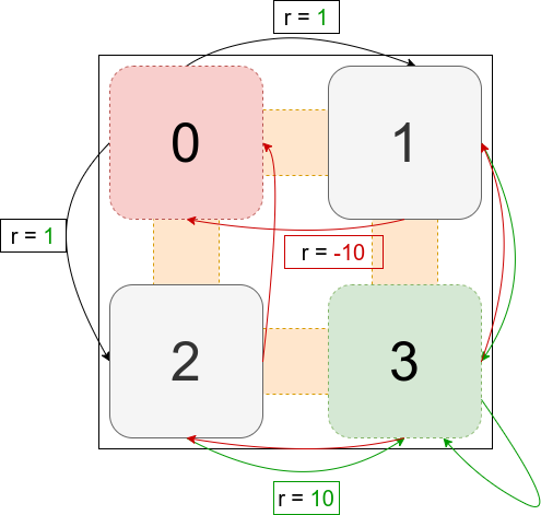
Here the process is still a MDP because it respects the assumptions under Markov Decision Processes. We ignore in our example the transition probabilities for simplicity and apply the algorithm for one step.

After one step, the optimal policy is the following:

$$ \begin{array}{l}V_1\ =\ \left[1,\ 10,\ 10,\ 10\right]\\\ \pi^* =\ \left\{\left[a_1,\ a_3,\ a_3,\ a_3\right],\ \left[a_2,\ a_3,\ a_3,\ a_3\right]\right\}\end{array} $$

Which absolutely makes sense, because in this MDP, to reach an optimal reward value you should avoid moving to the state $s_0$ and move to $s_3$ whenever you can.

Policy Iteration

Policy iteration is another algorithm to find the optimal policy when the transition probabilities and the reward function are known, the configuration of the problem is the same as before.

Instead of starting with an arbitraty Value function, we start the algorithm with an arbitrary policy $ \pi_0 $.

The main difference here is that for each step, the policy is supposed to be known. We can use the explicit Bellman Operator to calculate at each step the Value Function associated with the policy. Also, the policy is updated at each iteration where on the Value Iteration it is explicitly computed at the end of the algorithm.

This can be done only if the transition probabilities are known beforehand. What if we do not have access to them? The agent needs to learn by its own experience.

Monte Carlo for Policy Evaluation

How to figure out V for unknown MDP ( assume we get the policy)??

Assume we have a fixed policy $\pi$. We can estimate the value function empirically, by executing (from the same initial state) $n$ trajectories and estimating the Value function using: $$ \hat{V_n} (s_0) = \frac{1}{n} \sum^{n}_{i=1} \hat{R_i} (s_0) $$

With $\hat{R_i} (s_0)$ corresponding to the estimated reward of the trajectory $i$. A theorem ensures that the Monte Carlo estimator converges to the Value Function.

We saw that with this approach we can only estimate the value function for $s_0$. How do we estimate it for other states?

Every Visit Monte Carlo

After the $i$th trajectory, instead of updating only $s_0$, for all $k=T_i-1$ down to $0$: $$ \widehat{V}\left(s_{k, i}\right)=\widehat{V}\left(s_{k, i}\right)+\alpha_{i}\left(s_{k, i}\right)\left(\sum_{t=k}^{T_{i}} \gamma^{t-k} r_{t, i}-\widehat{V}\left(s_{k, i}\right)\right) $$

Temporal Difference Learning

TD(0) Estimation

At each state $s_t$ we observe the next state $s_{t+1}$ and the reward at the current state $r_t$. At this point, we compute the **temporal difference** as the weighted difference between the Value Function at the current state and the estimated Value Function at the next state. $$ \delta_t = r_t + \gamma \hat{V^{\pi}} (s_{t+1}) - \hat{V^{\pi}} (s_t) $$

The Value function at the state $s_t$ will be updated as the following:

$$ \hat{V^{\pi}}(s_t) = \hat{V^{\pi}} (s_t) + \alpha_t \delta_t $$

This is done for each episode (i.e. each predicted trajectory)