Model-free Reinforcement Learning

We previously saw various cases of how to solve an MDP when the MDP is given (i.e. known transition probabilities and reward function). Often the problems are not that simple, as we call them model-free. The agent will only have access to a black box interacting with him.

We saw in this case that we can solve the MDP using several techniques such as Monte Carlo learning, that looks at several trajectories and estimates the empirical Value Function, or TD(0) learning that bootstraps the reward function of the next states and computes the difference between the expect reward at the next state and the observed reward at the next state.

Model-free Prediction / Model-free Policy evaluation

Monte Carlo learning

The idea behind Monte Carlo learning si extremely simple. After getting $k$ trajectories, we estimate the Value Function by the expectation of the total discounted reward of each state. How do we update the Value Function for any state $s$?

First visit Monte Carlo

For each episode:

• In the first time step $t$ that state $s$ is visited in an episode:

• Increment counter $N(s) \mapsto N(s) + 1$
• Increment total return $S(s) \mapsto S(s) + G_t$
• Value is estimated by mean return $V(s) = S(s) / N(s)$
• By law of large numbers, $V(s) \mapsto V^{\pi} (s)$ as $N(s) \mapsto \infty$

We evaluate the state $s$ by taking into account the reward only for the first visit at each episode.

Every visit Monte Carlo

For each episode:

• Every time step $t$ that state $s$ is visited in an episode:

• Increment counter $N(s) \mapsto N(s) + 1$
• Increment total return $S(s) \mapsto S(s) + G_t$
• Value is estimated by mean return $V(s) = S(s) / N(s)$
• By law of large numbers, $V(s) \mapsto V^{\pi} (s)$ as $N(s) \mapsto \infty$

Incremental Monte Carlo

The mean of a sequence can be computed incrementally $$ \begin{equation*} \mu_k = \frac{1}{k} \sum_{i=0}^k x_i \end{equation*} $$ $$ \begin{equation*} \mu_k = \frac{1}{k} (x_k + \sum_{i=0}^{k-1} x_i) \end{equation*} $$ $$ \begin{equation*} \mu_k = \frac{1}{k} (x_k + (k-1)\mu_{k-1}) \end{equation*} $$ $$ \begin{equation*} \mu_k = \mu_{k-1} + \frac{1}{k} (x_k -\mu_{k-1}) \end{equation*} $$

For each episode:

• For each state $S_t$ with return $G_t$:

• $N(S_t) \mapsto N(S_t) + 1$
• $V(S_t) \mapsto V(S_t) + \frac{1}{N(S_t)} (G_t - V(S_t)) $

Temporal Difference Learning

• TD methods learn directly from episodes of experience
• TD is model free
• TD learns from incomplete episodes by bootstrapping
• TD updates a guess towards a guess

TD(0) algorithm

The idea is to update the value $V(S_t)$ toward the estimated return $R_{t+1} + \gamma V(S_{t+1})$

• V$(S_t) \mapsto V(S_t) + \alpha (R_{t+1} + \gamma V(S_{t+1}) - V(S_t))$

We want the estimated Value Function to update in the direction of the estimated immediate reward! Useful when the reward on the current state does not really depend on the result after doing a whole trajectory.

TD($\lambda$) algorithm

Let TD target look $n$ steps into the future! That is the main idea behind TD($\lambda$) algorithm. let us define the n-step return as the following:

• $n = 1$ $G_t^{(1)} = R_{t+1} + \gamma V(S_{t+1})$ (TD)
• $n = 2$ $G_t^{(2)} = R_{t+1} + \gamma R_{t+2} + \gamma^2 V(S_{t+2})$
• $n = \infty$ $G_t^{(\infty)} = R_{t+1} + \gamma R_{t+2} + … + \gamma^{T-1} R_T$ (MC)

Which $n$ is the best?

Bias / Variance trade-off

• TD target $R_{t+1} + \gamma V(S_{t+1})$ is biased estimate of $V^{\pi} (S_t)$
• TD target is much lower variance than the return (MC estimate).

TD vs MC

• TD can learn before knowing the final outcome

  • TD can learn online after every step
  • MC must wait until end of episode before return in known

• TD can learn without the final outcome

  • TD can learn from incomplete sequences
  • MC can only learn from complete sequences
  • TD works in continuing (non-terminating) environments
  • MC only works for episodic (terminating) environments

• MC has high variance, zero bias

  • Good convergence properties
  • Not very sensitive to initial value
  • Vary simple to understand and use

• TD has low variance, zero bias

  • Usually more efficient than MC
  • TD(0) converges to $V^{\pi} (s)$
  • More sensitive to initial value

Model-free Control / Model-free Policy learning

SARSA

How do we learn the best policy?? A family of methods that can be used is called Actor-Critic methods.

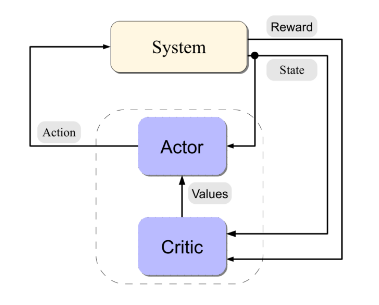
The idea here is that the two components act between each other, at each iteration $k$ the Critic evaluates the policy $\pi^k$ and the Actor improves the policy by acting greedily.

The Critic will use the TD learning to update the estimated Value function (or Q-function)

$$ \delta_{t}=r_{t}+\gamma \widehat{Q}\left(s_{t+1}, a_{t+1}\right)-\widehat{Q}\left(s_{t}, a_{t}\right) $$

$$ \widehat{Q}\left(s_{t}, a_{t}\right)=\widehat{Q}\left(s_{t}, a_{t}\right)+\alpha\left(s_{t}, a_{t}\right) \delta_{t} $$

Q-learning